This post is intended to give a more detailed explanation of the use of PID controllers in my two-wheeled robot project. I posted a series of articles about this project on the Dronebot Workshop forum over here. PID controllers are pretty much indispensable for robotics projects so I wanted to make sure that I dedicated a single article to them. There’s a very well documented Arduino PID library, which can be used for most projects, but I wanted to make sure that I had a good grasp on the subject hence the reason for rolling my own.
PID Controllers
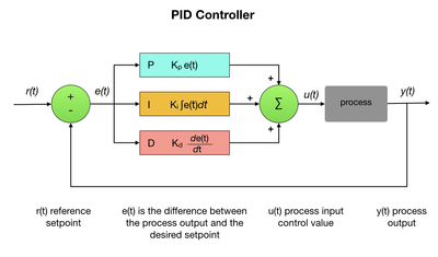
A PID controller is a control loop feedback mechanism that calculates the difference between a desired setpoint and the actual output from a process, and uses the result to apply a correction to the process. PID stands for Proportional, Integral, Derivative. The following diagram may look a little scary if your calculus is a bit rusty, but it’s really quite simple. The process’s job is to maintain a specified setpoint value. For example, you may want a DC motor to maintain a setpoint value r(t) of 600 encoder pulses per second. The actual motor speed y(t), called the process variable, is subtracted from the setpoint value 600 to find the error value e(t). The PID controller then computes the new control value u(t) to apply to the motor based off of the computed error value. In the case of a DC motor, the control value would be a Pulse Width Modulation (PWM) signal. The (t) part of this is just a time parameter that’s being passed into the process.
Here’s how each of the PID terms work:
P - proportional. This simply takes some proportion of the current error value. The proportion is specified by a constant called the gain value and for a proportional response is represented by the letters Kp. As an example, Kp may be set to 0.3 which will compute a value of 30% of the error value. This is used to compute the corrective response to the process. Since it requires an error to generate the proportional response, if there is no error, there is no proportional part of the corrective response.
I - integral. This takes all past error values and integrates them over time. Don’t be intimidated by the word integrate, it just means accumulate. This results in the integral term growing until the error goes to zero. When the error is eliminated, the integral term will stop growing. If an error still exists after the application of proportional control, the integral term tries to eliminate the error by adding in its accumulated error value. This will result in the proportional effect diminishing as the error decreases, this is compensated for by the growing integral effect.
D - Derivative. The derivative term is used to estimate the future trend of the error based on its current rate of change. It’s used to add a dampening effect to the system. The more rapid the change, the greater the controlling or dampening effect.
There are many control systems that do not require the use of all three PID terms. The P or I terms could be used by themselves or in the combinations PI or PD.
PID for Motor Control
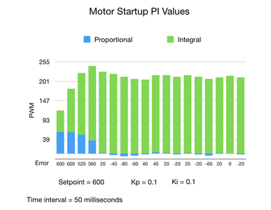
For motor control we only need to use the PI terms of the PID controller. Here’s a chart of the Proportional and Integral values of one of the motors on my two-wheeled robot project as it starts up.
I put the setpoint value to 600 encoder pulses per second, which will require the motor control input value to stay at around the 200 PWM mark. At the start, when the error is large, the Proportional term plays a significant roll in getting the motor up to the required setpoint speed. While this is happening the Integral part is accumulating the past error values eventually reaching total of around 200 PWM. At this point, the Proportional part drops to around zero and the Integral part does most of the work. A common behavior of PID control is that there can be a slight overshoot as we reach the setpoint before it settles down to a narrow range around the setpoint value. The Pl values will constantly adjust to take care of disturbances in the system. Notice that the Proportional value turned negative just after the initial overshoot to pull the system back down to within range of the setpoint value.
The Code
The following sample code implements a PID controller for a DC motor. For a PID controller to work properly it must be called at a consistent interval. Therefore, the function containing the PID algorithm should be called from a periodic timer interrupt. A DC motor can be controlled by using only the Proportional and Integral terms, so the Derivative term constant Kd is set to zero. The other constants Kp and Ki can initially be guessed at and later tuned to reach a satisfactory value. I’ve set them both to 0.1, which works satisfactorily on my robot and also makes it easy to understand the math.
The error is calculated by subtracting the current process variable, pulses per second in this case, from the required setpoint. The PID control algorithm then goes to work. The proportional part Kp is multiplied by the current error value. This will naturally go to zero as the error is eliminated. The integral part Ki accumulates as the error moves from the setpoint value to zero at which point it stops growing. The integral part is primarily responsible for holding the setpoint at the desired level as shown in the graph above. The derivative part Kd will track how fast we’re approaching the setpoint and provide a dampening effect to avoid a severe overshoot of the setpoint value. The derivative term is sometimes referred to as the “anticipatory control”, since it seeks to mitigate any sudden changes in the output control variable. I haven’t found it necessary to use the Kd term for controlling the motors, so I’ve set it to zero.
The sum of all three PID terms produces the motor control PWM variable. This becomes our process control variable, which is applied to the motor.
 // PI control. Adjust gain constants as necessary
const float Kp = 0.1, Ki = 0.1, Kd = 0.0; // gain constants

void setPowerISR() {

  // Get the number of pulses since the last period
  pulsesPerSec = getPulsesPerSecond();

  // Compute the error between requested pulses/sec and actual pulses/sec
  error = pulseSetpoint - pulsesPerSec;

  // PI control
  pPart = Kp * error; // Proportional
  iPart += Ki * error; // Integral
  dPart = Kd * (pulsesPerSec - pulsesPerSecLast); // Derivative

  // We've put the setpoint to zero, stopping the motors
  if (iPart < 0.0) {
    iPart = 0.0; // Don't let integral part go negative
  }

  // Compute the PWM
  PWM = int(pPart + iPart - dPart);

  // Apply the power with the PWM signal
  applyPower(PWM);
}
PID for Position Control
In this section we’ll be controlling the speed of a robot relative to its current position. The plan is to provide for a smooth startup of the motors at the beginning of the journey and then slowly wind them down as we get near the target position. To carry this out we’ll need to use the Integral term to start the robot moving and the Proportional term to slow it down. The following code shows the position loop, which executes until we drive the position error to zero. A timer has been implanted into it so as we get a consistent time interval of 50 milliseconds. We’ll also need to set a flag to indicate that we’re in the startup phase of our journey towards the destination.
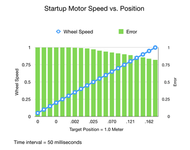
The startup operation is quite simple. We want to take the motor speed from zero to maximum speed within about one second. Since the time interval for our loop is around 50 milliseconds we set the Integral term of the PID controller to 0.05. This is then added into the iPart variable each time through the loop until we get to 1.0. At that point, we switch over to the running phase after which we set the wheel speed based on how far away we are from the target position.
As the robot nears the target position the Proportional part of the controller kicks in. The position error is being multiplied by the Kp constant and as it drops towards zero the result of that calculation gets smaller and smaller. It’ll quickly start trending towards zero where we would end up watching the robot creep towards its final destination in a painfully slow manner. To hurry things along we make sure that a minimum speed is maintained until we break out of the position loop and stop the motors.
The final part of the loop applies power to the motors, gets the robot’s current position, and recomputes the position error.
// Set min and max speed.
float maxSpeed = 1.0, minSpeed = 0.3;
float wheelSpeed = 0.0;
byte phase = STARTUP; // phase of the move
float iPart = 0.0; // PI values for start phase
const float startUpKi = 0.05;  // Ki value to startup robot
const float Kp = 3.0; // Gets within 20% of target

while (fabs(poseError[X_POS]) > 0.0) {

  // Process the loop every 50 milliseconds
  current_time = nh.now().toSec();
  while(nh.now().toSec() < current_time + poseLoopPeriod) {
      //wait 50ms
  }

  // --- Calculate the new control variable using PID

  // Build up to max speed over several time periods
  if (phase == STARTUP) {
    iPart += maxSpeed * startUpKi; // only need Integral part
    wheelSpeed = iPart;
  }
  else { // Reached max speed
    // Slows down when we get near the target position
    // Sets wheel speed proportionally to the position error
    wheelSpeed = (poseError[X_POS] * Kp) + (minSpeed * dir); // Kp = 3.0, minSpeed = 0.3
  }

  // Keep max speed to 1.0
  if (fabs(wheelSpeed) > maxSpeed) {
    wheelSpeed = (maxSpeed * dir); // Max 1.0
    phase = RUNNING; // Now in the running phase
  }

  // --- Apply control variable (actuates the wheels)
  robot->setWheelSpeeds(wheelSpeed, wheelSpeed); // left and right wheel

  // --- Read current process variable (gets the current x position of robot)
  float *currentPose = robot->getLocalPose();

  // --- Calculate the error
  Matrix.Subtract(refPose, currentPose, 3, 1, poseError);

} // End while loop

// Stop the wheels
robot->setWheelSpeeds(0.0, 0.0);  // Stop
The following chart shows the results from my two-wheeled robot as it starts up. The distance travelled to the target position, which is one meter away, is shown along the bottom. As you can see, the robot takes about six time periods before it even starts moving. However, after about one second it’s firmly on its way as it reaches its full speed. This is indicated by the decreasing error value, shown on the left, and the increasing position value at the bottom.
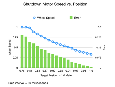
In the shutdown phase you can see the wheel speed being gradually pulled down as we near the target position. The process starts when we’re about 80% of the way to the target. This is probably a little premature but we can increase this to around 90% by increasing the Kp constant. As the position error goes to zero the motor speed drops to the minimum value of 0.3 where it remains until we break out of the position loop.
There’s a lot of information out there on PID controllers so I hope that this article has peeked you interest. If you have any questions, or I got anything wrong, please leave a comment.
@mjwhite - that is a most interesting post and it will take a while to fully digest. It comes as I'm just getting into the whole robot control subject so very relevant for me and appreciated.
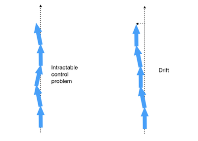
I was pondering the question of PID with navigation to a compass bearing. Lets say the bearing was due North to reach a destination point. The robot veers a bit to the left and the PID corrects to put it back to a North bearing. But, as some time was spent going left, to get back to the original destination point then the correction should be to send the robot to the right to correct the original veer to the left before again going on a Northerly track. Do you have any observations on this type of PID control?
I was not aware of the Arduino PID Library, again thanks for highlighting it, I will have to do a lot more research on this I can see.
Although the goal of getting the robot back onto the original track would be an ideal situation I don’t think it’s possible in practice. This is because of what’s called sensor noise where your sensors, whether they be encoders or an IMU, cannot ever give you a precise measurement of your actual location. A compass for example would not give you a reading of true north, especially in an indoor environment, since there would be various metal elements in the vicinity that would throw the measurement off. That’s one example of sensor noise. The bottom line is that once the robot has moved from its start position you can’t get back to the original track because you don’t know where the track is anymore.
Because of the sensor noise problem the best you can do is keep adjusting the robot to keep going straight ahead. However, you’ll always be off of the target position in the end. This is known as drift, and the further you go the more the drift.
The only way around this problem is to use localization where you use some external mechanism to determine where the robot actually is. There are multiple techniques for doing this and it’s a huge area of ongoing research. So welcome to the discussion.
If you get a chance would you mind explaining the idea that the robot never knows exactly where it is? Instead, it uses a series of noisy sensor measurements to estimate the probability of the location of the robot.
It is a key idea that is skipped over in hobbyist electronics. Based on your last couple of articles, I would guess you could do a great job introducing the intuition without getting too wrapped up in the math.
I’ll try to give an overview of the sensor noise problem. Sensor noise is a common problem in robotics that prevents you from knowing the exact position of the robot. There are basically two categories of position error, range error and drift error. Of the two, drift error is by far the biggest problem since small changes in orientation can produce large differences in the final X and Y position. This obviously gets significantly worse the further you go. The bottom line is that no sensor can accurately and consistently capture its surroundings. Here’re a couple of examples:
1) If a sonar signal bounces off of an angled reflective surface much of the signal won’t get echoed back to the receiver. Sometimes this will result in the object being detected and other times not. These readings can change wildly as the robot move. Also, if you have multiple sonars on your robot then some of the echoed signals can interfere with each other. This happens less often, but when is does it produces large discrepancies in the measurement.
2) A camera may return different visual information depending on such things as lighting and reflection. Moreover, this information can change even when the robot is not moving.
There’s also another issue compounding the problem of determining exactly where the robot is and that’s actuator noise. Think of a pair of wheels actuated with motors. The wheels may not be in perfect alignment, or they may undergo slippage during travel. Other issues may be uneven contact with the ground or inclines and declines. In that case, the encoder counts will not truly represent the distance and direction travelled.
It may be possible to separate out deterministic errors, such as uneven wheel alignment or the placement of an IMU, from non-deterministic errors, such as uneven lighting. In that case you could run a series of experiments to calibrate the robot, adding in a covariance value for use in your control calculations. Another possibility for mitigating position uncertainty would be to use multiple types of sensor in combination. For instance, you could use odometry (wheel encoders) together with dead reckoning (IMU). However, you would still experience drift over time and would need to turn to localization techniques at some point.
Thanks, mjwhite.
That is a good explanation that many beginner tutorials skip.

